Local realistic simulation of a Bell type experiment with two beams of equally polarized light.

Note: Light is considered a moving spread disturbance of a background medium. The disturbance can implement all of the features of  waves (intensity, wavelength, frequency, phase, polarization, phase speed, signal speed, etc) in such a way that within some local domain (of space and of time), well defined values of those wave magnitudes can be assigned to the local disturbance. Nothing new with that. It has been very well known for centuries.  But to understand what follows, the idea that light is made by localized particles (photons) must be rejected. The corpuscular behavior of light (in its interactions with matter) admits other explanations (not studied here) without the need to suppose that light itself is made of particles of specific energy, momentum, spin, etc.

Consider a source that at any given time emits light of equal linear polarization along two different directions (arms of the apparatus). The polarization direction itself of the emitted light varies with time in a random way.  

Suppose that there is at each arm of the apparatus a detecting device. The detecting device of each arm consists of a calcite (or more generally a polarization analyzer) and two identical photo-detectors. It will be admitted that the calcite splits its incident light in two beams of mutually perpendicular plane polarized light that go to their corresponding photo-detector.

It will be admitted that the intensities of both beams emerging from a calcite satisfy exactly Malus law. More precisely:

Let the calcite be oriented along direction z.

Let q be the angle that the direction of polarization of an incident light makes with the axis z. Then the intensity of light emerging from channel "up" of the calcite is I_o Cos²(q) while the intensity emerging from channel "down" of the calcite is I_o Cos²(q - p/2). Notice also that I_o Cos²(q) + I_o Cos²(q - p/2) = I_o

In each arm of the apparatus its photo-detectors will be labeled detector "up" and detector "down" (or more simply u and d) according to the beam (channel) of the splitter in which they are placed.

To simplify the analysis of the experiment it can be supposed that the light reaching the four photo-detectors is weak enough so that during the short time intervals in which these detectors are "open" they produce at most one click (i.e. only one ejected photo-electron starts the cascade). In these circumstances, it also seems reasonable to assume that there will be cases in which a photo-detector makes no click at all during some of the time intervals in which it is "open".

The name "count" will be used for a set of the 4 photo-detectors outputs (click or no-click) during a corresponding time interval (coincidence window) in which they are open to receive light. The four outputs of a count must correspond to observation intervals during which the four detectors are receiving light emitted by the source at the same epoch.

In respect to the output of the 4 detectors during a corresponding "count", the following 16 possibilities can therefore take place:

uu   dd   ud   du     u0    d0   0d   0u   00     u2    d2   2d   2u   22    02    20

where the first character of the pair refers to the output of the detectors of the first arm and the second character to the output of those of the second arm. The characters indicate the following:

u = the detector "up" of the corresponding arm makes a click (but not the "down" detector).

d = the detector "down" of the corresponding arm makes a click (but not the "up" detector).

0 = neither detector of the corresponding arm makes a click.

2 = both detectors of the corresponding arm make a click.

Counts (observations) are made at "all" possible relative angles of the two calcites. The angle that the "significant" axis of the second calcite makes with the "significant" axis of the first will be called F. The fact that the lights reaching the calcites during a corresponding count are supposed to have the same plane polarization direction implies therefore that if such light makes an angle q with (the significant axis of) the calcite of the first arm, it makes an angle q-F with the significant axis of the calcite of the second arm.

A computer simulation has been made in which it has been supposed (for simplicity and without loss of generality) that the first calcite is in all observations oriented along the direction z while the second calcite is oriented relative to the first (and therefore relative to the direction z) at an angle F that can be chosen at will. As said above, in "correspondence" with Malus law, it has been supposed that, for an incoming light polarized along direction q (relative to z), the probabilities of click of the 4 detectors are respectively:

Detector up of the first arm Cos²(q)                                                       [BE-1u]

Detector down of the first arm Cos²(q - p/2)                                         [BE-1d]

Detector up of the second arm Cos²(q - F)                                           [BE-2u]

Detector down of the second arm Cos²(q - F -p/2)                              [BE-2d]

For example, a simulation has been made making 20,000 counts for each of the 33 following relative orientations of the calcites: F = {0, p/64, 2p/64, 3p/64, … , p/2}. In each of the 33 x 20,000 counts the direction of polarization q of the light reaching both calcites has been assumed to take a fresh random value (giving an equal probability to all the directions between q = 0 and q = p).

For any given "count", the click occurrences of the four detectors have been implemented by the program as follows:
- As just said, first a fresh direction q (the same for both arms) is randomly obtained.
- Next, four random numbers between 0 and 1, (i.e. a fresh random number for each detector) are obtained that are compared with the classic (Malus) light intensity reaching the corresponding photodetector at its particular orientation relative to the direction of polarization q of the incident light:

Suppose for example that the four detector’s random numbers of a given count are respectively {0.987,  0.022,  0.561,  0.842}

The detector up of the first arm makes a click if and only if              0.987 £ Cos²(q)

The detector down of the first arm makes a click if and only if         0.022 £ Cos²(q - p/2)

The detector up of the second arm makes a click if and only if         0.561 £ Cos²(q - F)

The detector down of the second arm makes a click if and only if     0.842 £ Cos²(q - F -p/2)

-----------------------

The following table collects the results of a simulation made with Visual-Basic 6.0 and its Rnd (random) function.

Table [BE-3]

(The last row, labeled S, presents the sums of the respective columns).

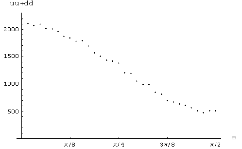
The following graphic plots the number of counts with "coincidences" as a function of the angle F between the calcites.

1) considering coincidences only those counts in which the output is either uu or dd (i.e. only the first two columns of the table):

                            Fig [BE-1]

Defining the correlation function (at a given relative angle F between the calcites) as:

                        [BE-3]

the above simulation gives the following plot:

                         Fig [BE-2]

2) considering coincidences, in a non strict way, all those counts in which the output is either uu, dd, u2, d2, 2u, 2d, 22 (i.e. in which detectors of the same kind (u or d) click in both arms including those cases in which both detectors of the same arm simultaneously click), the above simulation gave the following plot:

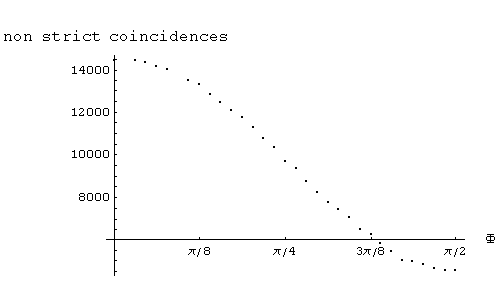            Fig [BE-3]

Note: if in the above "non strict coincidences", those cases/counts (labeled 22) in which the four detectors click simultaneously are counted twice, a very similar plot to Fig(BE-3) is obtained.

Comments:

1) - I did not had access to any of the famous articles (e.g. those of J.F. Clauser or A. Aspect) describing the Bell type experiments with singlet "paired photons" showing the violation of Bell’s inequalities and I only have indirect information about their results. (An important part of my information about the experiments and controversies related with EPR and Bell tests comes from reading the interesting critical articles of Caroline H. Thompson http://users.aber.ac.uk/cat/ )

If I understood correctly, when the Bell testers plot their experimentally obtained coincidences and/or correlations they obtain "cosine type" curves that seem to be a signature of violation of Bell’s inequalities. The above plots of this article are also "cosine type" curves. Furthermore, when the so called CHSH69 test is applied to the correlations obtained in the above simulation it gives:

Calling two specific calcite orientations of the first arm of the apparatus: a and a’

Calling two specific calcite orientations of the second arm of the apparatus: b and b’

For example, choosing for a, a’, b, b’ the following values (commonly used in these kinds of Bell tests):

                        Table [BE-4]

Calling C(p,q) the correlation function measured (or in this case predicted by the simulation) when the 1^st calcite is oriented along direction p and the 2nd along direction q, the CHSH test requires to measure the value of

S = C(a, b) - C(a, b’) + C(a’, b) + C(a’, b’)

And considering that for any pair of orientations p, q of the calcites the correlation results with polarized light do only depend on their relative orientation F=|q-p| , using the settings of the above Table [BE-4]:

S = C(a, b) - C(a, b’) + C(a’, b) + C(a’, b’) = C(0, p/8) - C(0, 3p/8) + C(p/4, p/8) + C(p/4, 3p/8) =

= C(p/8) - C(3p/8) + C(p/8) + C(p/8) =

and substituting the values obtained in the above simulation (that can also be read from Fig[BE-2]):

= 0.6373 - (-0.6138) + 0.6373 + 0.6373   =   2.5257

But the CHSH form of Bell’s inequalities states that (whatever orientations a, a’, b, b’) the correlations obtainable from local realistic models must obey

-2 £  C(a, b) - C(a, b’) + C(a’, b) + C(a’, b’) £  2

but the model of light simulated above is local and realistic and violates such relation. A local (hidden variables) reality can under some reasonable suppositions violate Bell’s inequalities. Therefore "Bell theory of non-locality (and therefore experimental Bell-type tests) does not have general validity because the theory makes wrong assumptions about the necessary features of local realistic models".

I (and many others) consider for example a wrong assumption to suppose that light is made of photons (i.e. localized particles). If this wrong assumption is made it must also be assumed that when a photon (one of the "entangled" pair emitted by the source) reaches a calcite it must take either one or the other of the two possible paths leading to the u or d detectors. It can not, according to the orthodox concept of photon, take both paths and trigger both detectors. It can neither disappear without triggering any of the detectors. Making that wrong assumption it can indeed be reasoned (in the line of Bell's theoretical reasonements) that a local realistic photon can not violate Bell's inequalities. (Simulation 2, below, reinforces such assertion). But instead, as the above simulation shows, it can also be reasoned that with a non-photonic but otherwise local realistic model of light, the Bell inequalities can be violated.

Simulation 2.

Another computer simulation with these "photon" assumptions has been made:

For any given "count", the click occurrences of the four detectors have now been implemented by the program as follows:

- First, a fresh polarization direction q (the same for both arms) is randomly obtained.
- Next, only two (instead of four) random numbers between 0 and 1, (i.e. a fresh random number for each arm) are obtained that are compared with the classic (Malus) probability that the photon takes the path "up" of the corresponding calcite at its particular orientation (relative to the direction of polarization q of the incident light):

Suppose for example that the two calcite’s random numbers of a given photon pair are respectively {0.874, 0.369}

The detector up of the first arm makes a click if and only if              0.874 £ Cos²(q)

The detector down of the first arm makes a click if and only if       0.874 > Cos²(q)

The detector up of the second arm makes a click if and only if         0.369 £ Cos²(q - F)

The detector down of the second arm makes a click if and only if  0.369 > Cos²(q - F)

With the same definition of the correlation function  

a typical photon model local realistic simulation gives instead the following plot:

                      Fig [BE-5]

The CHSH test now gives

S = C(a, b) - C(a, b’) + C(a’, b) + C(a’, b’) =

   = C(p/8) - C(3p/8) + C(p/8) + C(p/8) =

   =  0.3512 - (-0.3597) + 0.3512 + 0.3512   =   1.4133

that now obeys    -2 £  S £  2  therefore contradicting the experimental facts.

Summarizing:

A wave type disturbance (spread in space) model of light can be assumed to have a strictly locally defined polarization and can be assumed to trigger or not the photo-detectors according only to local conditions. (See the end of Section 6 of my @ether model http://personales.ya.com/carlosla/model/EVA6/Eva6.htm where I try to explain that the photo-detectors are triggered if the intensity of the light disturbance is "bigger" than that of the local @ether noise). This local realistic model of light can (in principle) explain the experimental Bell's inequalities violations without the weirdness of non-locality

If instead a photon type (localized in space) model of light is assumed to have a strictly locally defined polarization it can be reasoned and predicted (as Bell does) that it will obey Bell's inequalities and therefore will be unable to explain the experimental facts.

The theoretical analysis (and conclusions about non-locality) of Bell (and followers) do not have a general validity.

 Simulation 3. With reduced photo-detector’s efficiencies.

28-Mar-2003. Having posted a summary of the above results to the Yahoo group qm2 http://groups.yahoo.com/group/qm2/ , Caroline H. Thompson made several comments and suggestions one of which was:

Before going much further, how about doing the following:

(a) Run the model simulating imperfect detectors.  To make it possible (in
theory) to check the results, do this by first using your Malus' Law method
then throwing away the count with probability (1 - e), where e is the
"efficiency".  You should, if I'm right, find that when you have very low
efficiency (as in real experiments) you can no longer violate your test …

My first thought was to answer:

Well, …, if I suppose in my simulations that the "efficiency" e of the photo-detectors is independent of the intensity of the radiation that they receive this should have no influence in the violation or not of the test that I have so far simulated, because such supposition would only have the effect to multiply the number of counts of the types uu, dd, ud and du by the same constant value e². Therefore the correlation function that I have been using (uu+dd-ud-du)/(uu+dd+ud+du) would be the same as before (at any given relative angle) whatever the efficiency e.

But, just in case my intuition was wrong I made the simulation suggested by Caroline and: Caroline is right. Here is the result of the simulation suggested by Caroline:

I chose an "efficiency" e = 0.4 (the same of course for the four photo-detectors). As above the program samples 20,000 times (counts) each relative angle of the calcites. For each count:

- first a fresh direction q (the same for both arms) is randomly obtained.
- next, four random numbers between 0 and 1, (i.e. a fresh random number for each detector) are obtained that are compared with the classic (Malus) light intensity reaching the corresponding photo-detector at its particular orientation relative to the direction of polarization q of the incident light.

Suppose for example that the four detector’s random numbers of a given count are respectively {0.987, 0.022, 0.561, 0.842}

The detector up of the first arm makes a pre- click if and only if              0.987 £ Cos²(q) . e

The detector down of the first arm makes a click if and only if         0.022 £ Cos²(q - p/2) . e

The detector up of the second arm makes a click if and only if         0.561 £ Cos²(q - F) . e

The detector down of the second arm makes a click if and only if     0.842 £ Cos²(q - F -p/2) . e

Note: this way of deciding the click/no-click multiplying the Malus intensities by the efficiency e and comparing the product with the random number has the same effect (i.e. produces the same distribution of counts) as the routine suggested by C.H.T.   that consists in "throwing away the count with probability (1 - e)" doing the following : (for example with the detector u of the first arm): If   0.987 > Cos²(q) consider it straight away a no-click and go to deduce the event of the next detector. But if 0.987 £ Cos²(q) consider it a candidate for a click and find another random number r (again between 0 and 1) . If r > (1-e) then consider it a click and otherwise a no-click, and go to deduce the event of the next detector. (In spite, I insist, that as I have checked, this second routine produces statistically identical results, I feel more comfortable with the first that depends on only one random "event").

                Fig [BE-6]

Using the same definition of the correlation function     

                    Fig [BE-7]

The CHSH test now gives

S = C(a, b) - C(a, b’) + C(a’, b) + C(a’, b’) =

   = C(p/8) - C(3p/8) + C(p/8) + C(p/8) = 1.767 < 2

and therefore, as Caroline predicted, the test is no longer violated (for this example detector efficiency e=0.4)

Trying to understand where failed my intuition I compare the absolute number of counts of the types uu,dd,ud,du of the first test with those of this latter   "reduced efficiency test" that I label with upper case letters UU, DD, UD, DU in the following table:

 Table [BE-8]

Note: Other simulations and corresponding CHSH correlation tests have been made supposing other detector efficiencies (together with linear response of the detectors with light intensity). Here are some examples:

e = 0.2             S = 1.79

e = 0.6             S = 1.94

e = 0.8             S = 2.25

where, as above,     S = C(p/8) - C(3p/8) + C(p/8) + C(p/8)

Analytical expressions for the predicted uu, dd, ud, du counts in these type of Bell type experiments supposing a classic non-photonic model of light.

Again Caroline H. Thompson ( http://users.aber.ac.uk/cat/ ) has found an easy way to calculate analytical expressions for the predicted uu,dd,ud and du counts at any given orientations a, b of the polarizers (e.g. calcites) and for any given "efficiency" e of the detectors. It goes like this:

Let q be the common direction of polarization of the light reaching both polarisers. Consider a polariser set at angle z:

- the probability that the "up" detector of the polariser triggers is Cos² [q - z]

- the probability that the "down" detector of the polariser triggers is Cos² [q - z - p/2] = Sin² [q - z]

and therefore the probability that it does not trigger is 1 – Sin² [q - z]

- therefore the joint probability of detecting "u" but not "d" at that polariser is

F(q, z) = Cos² [q - z] (1 – Sin² [q - z])

If the efficiency e of the detectors is smaller than 1, then such joint probability can be generalized by the following function:

F(q, z, e) = e.Cos² [q - z] (1 – e.Sin² [q - z])

Consider now both polarisers: F(q, a, e) F(q, b, e) is the joint probability to get a "u but not d" at polariser#1 (when set at angle "a") together with a "u but not d" at polariser#2 (when set at angle "b") and it is therefore the probability to get a count uu at those angle settings of the polarisers.

Note: As Caroline explained me, "the count uu now depends on the
integral of the product F(x, a, e) * F(x, b, e).  There is no neat factor
such as e*(1-e) that is going to factor out and cancel in your estimated
quantum correlation, (uu + dd - ud - du)/(uu + dd + ud + du).  e is
inextricably built into the function". 

That explains why failed my intuition, as mentioned above.

The expected number of uu counts in a big number n of trials in which the direction q of the "paired" light entering the polarisers varies randomly (with equal probability to fall between 0 and p) is

that once integrated gives

             [BE-8a]

(By symmetry the expected number of dd counts is at all angle settings of the polarisers equal to the expected number of uu counts, i.e. N[dd] = N[uu] )

Similarly the probability to obtain a d (but not u) in any one of the polarisers is :

G(q, z, e) = e.Sin² [q - z] (1 – e.Cos² [q - z])

The probability to, again, obtain a u (but not d) in the other polariser is as above:

F(q, z, e) = e.Cos² [q - z] (1 – e.Sin² [q - z])

And the joint probability to obtain a du count when considering both polariser is therefore:

G(q, z, e) F(q, z, e) . Therefore the expected number of du counts in a big number n of trials in which the direction q of the "paired" light entering the polarisers varies randomly (with equal probability to fall between 0 and p) is

that once integrated gives

             [BE-8b]

(By symmetry the expected number of du counts is at all angle settings of the polarisers equal to the expected number of ud counts, i.e. N[du] = N[ud] )

It can be checked that these analytical expressions N[uu], N[dd], N[ud], N[du] agree very satisfactorily with the results of the above simulations given in Table[BE-3] and Table[BE-8]

The correlation function defined as

C(a,b;e) = (N[uu]+N[dd]-N[ud]-N[du]) / (N[uu]+N[dd]+N[ud]+N[du])

takes the expression:

                                           [BE-8c]

and the result of the CHSH69 test is related with the efficiency of the detectors by:

            [BE-8d]

Comments:  Vladimir Z. Nuri (founder of the Yahoo qm2 discussion group) that has been insisting for a long time in several  forums on the importance of the efficiency issue in the analysis of Bell-test experiments has commented that our above expression [BE-8d] and graphic predicts that it is for high efficiencies that the Bell inequalities should be violated in contradiction with the well known fact that in many Bell test experiments the detector efficiencies are very low in spite of which the inequalities are experimentally violated. (It must be added that Vladimir judges nevertheless very positively the significance of this study). Caroline H.T. has argued that the result obtained above is a different matter from the usual detection loophole in which the cause of the high S value could be ascribed to the nonlinearity of detection. I agree with the interpretation of Caroline H.T. as suggests the following Simulation 4:

-----------------------------------------------

Simulation 4:  with non linear response of the photo-detectors to intensity

Suppose that at very low light intensities (like those used in many "single photon" Bell tests experiments) the probability that a photodetector "ejects" (during any of its open intervals) a photo-electron is not directly proportional to the intensity of the light entering its window. It can then be seen that, for "reasonable" non linear relations between the intensity and the probability of photodetection, the simulation again predicts the violation of Bell’s inequalities. Suppose that the photo-detectors behave according to the following relation between the intensity I illuminating them and the probability of P(I) of photodetection (triggering):

                           Fig[BE-8]

And suppose an experiment in which the maximum intensity that the photo-detectors happen to receive is I_o (corresponding to the case in which the light entering the analyzer (e.g. the calcite) happens to be polarized parallel to one of the two "axes" and therefore the photodetector of the corresponding channel receives an intensity I_o Cos²(0) = I_o while the other receives none). If the detectors will only receive light intensities between 0 and I_o they will be working in the red part of the above curve that can be roughly approximated by the following (non linear) relation:

                                                             [BE-8]

that somehow means that in that experiment the efficiency of the detectors is at most e=0.35 Nevertheless, in apparent contradiction with the result of the above Simulation 3, now the simulation with these non linear detectors gives:

                Fig[BE-9]

                    Fig[BE-10]

And the CHSH test gives

S = C(p/8) - C(3p/8) + C(p/8) + C(p/8) = 2.65

The concept of quantum efficiency applies to detection of particles and is indeed very well defined and a very straightforward concept (i.e. the quotient between the number of detected particles and the number of particles that have entered the surface of the detector). If what enters the detector are indeed real particles (as opposed to light and other types of spread waves) it seems evident that in the case of a weak input of particles (no more than one particle entering the detector in a time interval long enough for the detector to "relax") the detector will behave the same whether the earlier particle entered 1 second or one year ago. I.e. the quantum efficiency is then independent of intensity and therefore linearity can be assumed at low intensities. But in the case of wave-like disturbances (or light pulses) entering a photo-detector the number of clicks per photon worth of energy of radiation can instead be expected to depend strongly on the intensity of radiation entering the photodetector. As long as one believes in "photons" as localized particles there is no reason to suspect that there might be a problem. I believe that is why in Bell experiments, no paper (that I know of) seems to analyze these aspects of the efficiency loophole.

Simulation 5

Caroline H. Thompson showed interest in knowing the result if I  "Modify the program to simulate what Weihs' et al  probably did, i.e. every time you get, for example, u2, allocate a count to either ud or uu at random".

This simulation 5 does that supposing:

- detector's efficiency e = 1 (and linear response to intensity).

- a count u2 is considered randomly either a uu or ud (each with 50% probability)

- a count 2u is considered randomly either a uu or du (each with 50% probability)

- a count d2 is considered randomly either a dd or du (each with 50% probability)

- a count 2d is considered randomly either a dd or ud (each with 50% probability)

- a count 22 is considered randomly either  uu, ud, dd, du   (each with 25% probability)

CHSH test:  S = C(p/8) - C(3p/8) + C(p/8) + C(p/8) = 1.83

Doing the same with detector efficiencies    e = 0.4
(graphics omitted)
CHSH test:  S = C(p/8) - C(3p/8) + C(p/8) + C(p/8) = 1.61

Return to the Home Page